Seafloor magnetic stripes: look again
In the mid 1960s, evidence of magnetic stripes on the seafloor convinced the geologic community of the validity of plate tectonics theory, and it is often pointed to today as clinching evidence for the theory. The public has not heard anything new about this pivotal find. It is time to look again.
The Geodynamo
Without seeing into the center of the Earth, we cannot know with certainty the source of the geomagnetic field. The current thinking is explained by Dr. Gary A. Glatzmaier, Professor of Earth Sciences at UCSC, Santa Cruz, on the geodynamo page of his website. His work on computer modelling in the mid-1990s demonstrated how polarity reversals might occur in the geodynamo. Quoting him (my emphasis in blue):
"Paleomagnetic records indicate that the geomagnetic field has existed for at least three billion years. However, based on the size and electrical conductivity of the Earth's core, the field, if it were not continually being generated, would decay away in only about 20,000 years since the temperature of the core is too high to sustain permanent magnetism. In addition, paleomagnetic records show that the dipole polarity of the geomagnetic field has reversed many times in the past, the mean time between reversals being roughly 200,000 years with individual reversal events taking only a couple thousand years. These observations argue for a mechanism within the Earth's interior that continually generates the geomagnetic field. It has long been speculated that this mechanism is a convective dynamo operating in the Earth's fluid outer core, which surrounds its solid inner core, both being mainly composed of iron. The solid inner core is roughly the size of the moon but at the temperature of the surface of the sun. The convection in the fluid outer core is thought to be driven by both thermal and compositional buoyancy sources at the inner core boundary that are produced as the Earth slowly cools and iron in the iron-rich fluid alloy solidifies onto the inner core giving off latent heat and the light constituent of the alloy. These buoyancy forces cause fluid to rise and the Coriolis forces, due to the Earth's rotation, cause the fluid flows to be helical. Presumably this fluid motion twists and shears magnetic field, generating new magnetic field to replace that which diffuses away. However, until now, no detailed dynamically self-consistent model existed that demonstrated this could actually work or explained why the geomagnetic field has the intensity it does, has a strongly dipole-dominated structure with a dipole axis nearly aligned with the Earth's rotation axis, has non-dipolar field structure that varies on the time scale of ten to one hundred years and why the field occasionally undergoes dipole reversals. In order to test the convective dynamo hypothesis and attempt to answer these longstanding questions, the first self-consistent numerical model, the Glatzmaier-Roberts model, was developed. Our solution illustrates how the influence of the Earth's rotation on convection in the fluid outer core is responsible for this magnetic field structure. About 36,000 years into the simulation the magnetic field underwent a reversal of its dipole moment, over a period of a little more than a thousand years. The intensity of the magnetic dipole moment decreased by about a factor of ten during the reversal and recovered immediately after, similar to what is seen in the Earth's paleomagnetic reversal record. Our solution shows how convection in the fluid outer core is continually trying to reverse the field but that the solid inner core inhibits magnetic reversals because the field in the inner core can only change on the much longer time scale of diffusion. Only once in many attempts is a reversal successful, which is probably the reason why the times between reversals of the Earth's field are long and randomly distributed. After the first magnetic reversal, we continued our simulation." Using "a heterogeneous heat flux similar to the Earth's present pattern", the model "underwent two more reversals, roughly 100,000 years apart. This demonstrates the influence the thermal structure in the lower mantle has on the style of convection and magnetic field generation in the fluid core below.The popular story
The general impression is that nice, even bands of alternating polarized rock form as new seafloor is made by the slow, steady movement of plates over millions of years and regular reversals of the geomagnetic field about every 200,000 years. It is often illustrated with this kind of diagram, which I call 'piano keys':
Reality
The stripes themselves are better described with words like irregular, blobbed, marbled, blended, meandering, as if shaken while in a fluid state and divided by segments diverging along transform faults.
On the left below is the familiar global map of the age of the sea floor using presumed magnetic isochrons. See how even the bands are. On the right is a global map of sea floor spreading rates, based on the measurable width of rock segments. What plate tectonic forces do you suppose caused such jerky movement in many individual segments? The chaotic jumble on the right in many areas should be matched on the left, but it has been nicely smoothed out.

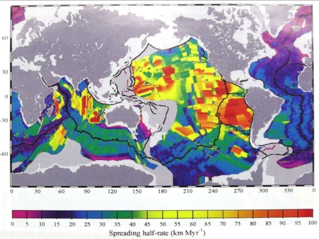
From
McElhinny, Michael W., Phillip L. McFadden, Paleomagnetism: Continents
and Oceans. 2000. Academic Press, San Diego, CA.
Maps opposite
pages 206 and 207
Now look at the frequency of reversals (data from Cande and Kent, 1995).
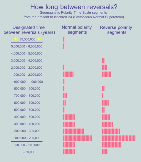
As Dr. Glatzmaier wrote, the mean frequency of reversals is about 200,000 years. How many would you expect to be within, say, 50,000 years of 200,000? It is 19% (35 of 185), only one-third of what one would expect in the standard normal distribution. The reversals lie primarily between 30,000 and 500,000 years, with another spike at 1,000,000 to 2,000,000 years and a significant number across the rest of the spectrum. Rather than a regular tempo of reversals, it instead seems fairly chaotic. And what does the supposed 35 million year "Cretaceous Normal Superchron" represent? One would expect over 150 reversals in that period of time, but there are none. "Assuming the probability of a reversal to be constant with time, the lengths of polarity chrons should be distributed exponentially. In fact the distribution of observed polarity chrons is not exponential but contains too few short chrons."(Lanci, 1997) Earth's magnetic field might occasionally reverse as Dr. Glatzmaier has described, but perhaps that is not what the magnetic stripes have recorded.
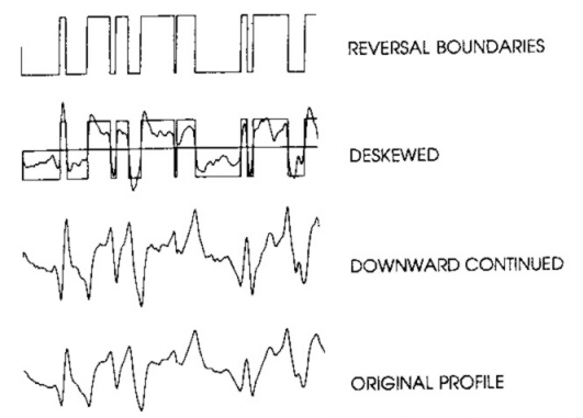
Consider the data itself. Ships or submersible vessels make a number of passes over a region of ocean floor, recording magnetic anomalies. The profiles are displayed down the page in a 'stack'. Then lines are drawn from profile to profile where the researcher guesses common points exist.
William W. Sager,
Chester J. Weiss, Maurice A. Tivey, H. Paul Johnson. March 10, 1998.
Geomagnetic polarity reversal model of deep-tow profiles from the
Pacific Jurassic Quiet Zone. Journal of Geophysical Research, Vol.
103, No. B3, pp. 5269-5286.
A test
In 1993, these profiles (traces) reminded a doctor of math and statistics of something he had seen before. He found their appearance to be "quite similar to what in harmonic analysis is called band limited noise. In other words, the traces look like the result of some system that is varying randomly but is constrained to vary neither too slowly nor too quickly with distance." "It is known that a fairly irregular fine-grained variation can be made to appear coarser and more regularly varying by averaging over local regions." "If this could be the case, what could be causing the averaging? The clear candidate here is the measurement process itself. The intensity measurements are (generally) made from surface vessels which travel several kilometers above the ocean floor, and more above the basement rock. The intensity measured at any surface point is thus actually the (weighted) average effect of the intensities in the basement rock for a horizontal distance of several times the vertical distance to the measuring device. This is indeed about the width of the anomaly peaks in the intensity traces."(Smith, 1993)
He next used a computer to randomly generate a sequence of magnetic polarity values with closer spacing than actual magnetic anomalies. "Variations of grain size and the nature of the random generating process did not make much difference in the appearance of the resulting traces. The fine variation was then filtered by a model of the measurement process." "Four traces were simulated using different seeds for the random generator."(Smith, 1993) Finally, he compared the simulation with examples of real profiles: "The general appearance of the simulated traces is quite similar to the observed traces. The peaks have about the same degree of regularity in both. Degree of variation in peak shape is similar in both." With one exception, "the correlations between the random simulated traces are of about the same quality as those between the observed traces. In both, individual peak shape is of little use in correlation. In both, to achieve a one-to-one peak correspondence, the peak counts must be fudged a little by counting minor peaks where necessary or by lumping some somewhat distinct peaks into one. In both, there are regions of little obvious similarity. In both, pronounced correlations between peak groups 'fizzle out' upon passing to yet other traces."(Smith, 1993)
Smoothing the profiles
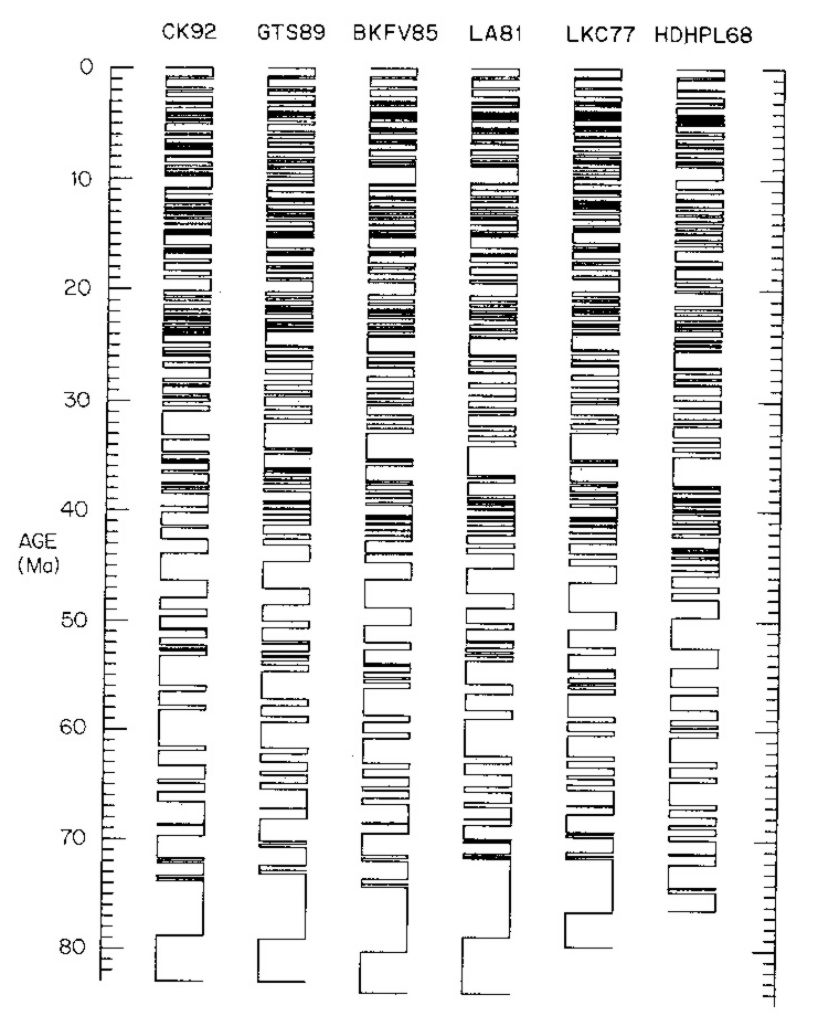
Here is how the ambiguous data of the profiles is processed by researchers to produce the simple black and white binary stripes that Plate Tectonics expects. These three figures are from the Journal of Geophysical Research.(Cande, 1992)
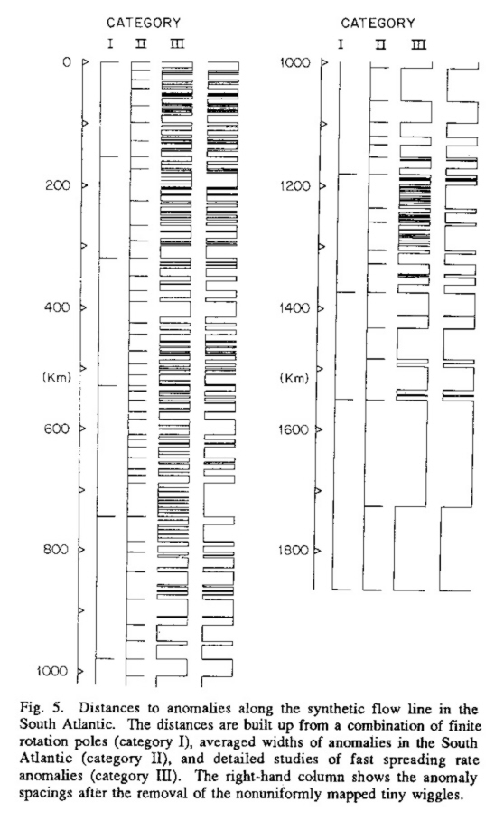
This is a remarkable comparison. Each column is a timescale produced by different people for the same time period. With so much processed data, one would expect more agreement.
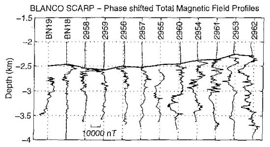
Vertical changes
Magnetic polarities also vary with depth. In the late 1990s, a team of investigators "used the submersible ALVIN to collect near-bottom magnetic profiles up a steep scarp face that exposes upper oceanic crust. The survey focused on the Blanco Scarp... in the northeast Pacific."(Tivey, 1998) They measured magnetic anomalies down to about 3.5 km. Apparently half to three-quarters of the recorded magnetic anomaly comes from the upper 3.5 km of oceanic crust, consisting of upper pillow lava and lower lava.(Tivey, 1998) These are the readings. Each vertical dotted line is zero, and polarity is measured by the distance the line shifts to the left or right of zero.
This is the interpretation, which simply places the measurements on a cross-section of the scarp. Swings to the right are in black, to the left in white. It confirms findings from deep sea drilling as far back as 1979 (Hall, 1979) that magnetic polarity changes direction at different depths.
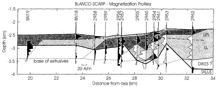
To explain it, the authors suppose that lava is extruded not only in the center of a spreading ridge but along its sides as well, up to 3 km. There is clearly considerable variation over short distances, both vertically and horizontally, with no indication of the smallest unit of measure in either dimension. "While lateral variability in polarity structure is correlatable at ~0.5-1 km profile spacing, magnetization intensity appears to vary on a smaller length-scale and is likely to be ultimately of a fractal nature."(Tivey, 1998) That means the measurement process is still averaging the randomness that Dr. Smith found.
A dyke is a sheet of magma that has risen up through a crack in rock strata. The Lhasa Block is at the center of the collision between India and Asia that raised the Himalayas. A study that took samples from a dyke in the Linzhou basin of the Lhasa Block revealed a polarity reversal. "Samples from one and the same dyke show both normal and reverse polarity directions." "The results of this study indicate that the antipodal remanence directions separated from dyke samples in the Linzhou basin are due to different polarities of the Earths magnetic field rather than resulting from a self-reversal process." In this region, "the thickness of the dykes varies from about 1.5 to 10 meters." The magma had to rise all the way through the crack at one time; if it had stopped part way, it would have blocked the magma below from rising further. Samples were taken near the surface; there may be more at depth. The researchers estimated "cooling times of maximum 500 years (time until the maximum temperature in the dyke has reached 100 Centigrade)." (Liebke, 2012)
Tiny wiggles
The clean pattern of reversals sought for Plate Tectonics is complicated by so-called 'tiny wiggles' or 'cryptochrons'. "Marine magnetic anomalies generally have high amplitudes (~300-500 nT) and long wavelengths (~100-200 km), depending on spreading rate and polarity chron length. However, marine surveys over fast spreading oceanic crust have shown that the magnetic record also contains lineated anomalies with low amplitudes (25-100 nT) and short wavelengths (8-25 km). These small features were dubbed 'tiny wiggles'. The small-scale anomalies can be traced between parallel profiles and are found to be contemporaneous in different ocean basins."(Lanci, 1997) There has been disagreement over the years as to the cause of the tiny wiggles, but a concensus seems to be forming that they are related to changes in the intensity of the geomagnetic field rather than its polarity.(Lanci, 1997; Gee, 1996)
Excursions
Two detailed "studies of the geomagnetic field in the last 1 million years have found 14 excursions, large changes in direction lasting 5-10 thousand years each, six of which are established as global phenomena by correlation between different sites. The older picture of the geomagnetic field enjoying long periods of stable polarity may not therefore be correct; instead, the field appears to suffer many dramatic changes in direction and... reduction in intensity for 10-20 percent of the time." "Intervals of constant polarity are called chrons". "Excursions take place within these intervals" and are shorter than chrons. "The magnetic direction departs greatly from the usual geocentric axial dipole, sometimes achieving the reverse direction for a short time." "Excursions also involve dramatic decreases in intensity." They "involve a rapid collapse of the field". These results "paint a quite new picture of geomagnetic behavior. Excursions appear to be a frequent and intrinsic part of the (paleomagnetic) secular variation".(Gubbins, 1999)
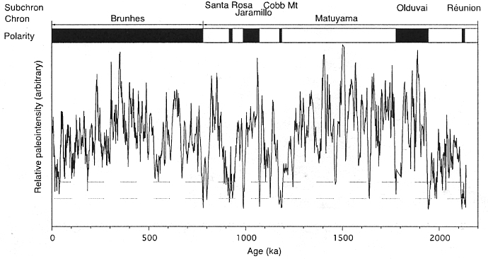
Geomagnetic
reversals and relative paleointensity variations for the last 2.14
million years. Polarity bar along the top: black is "normal",
white is "reversed".(Roberts, 2008)
"The geomagnetic field is dynamic, with constantly changing paleointensity and abundant collapses, when excursions are more likely to occur."(Roberts, 2008)
One study describes an excursion as "an 'aborted' polarity surrounded by two reversals." "The term 'aborted' results from the fact that this period should not be regarded as a real polarity state." "Below a certain strength the field reaches an unstable position which" leads to either "a reversal or its return to the former polarity." "One then wonders why the field is occasionally able to complete a reversal and generate a new polarity state, while it goes backward in the other cases (excursions)." "Scarcity of sedimentary and volcanic records of excursions indicates that they are indeed very short events, on the order of a few thousand years at most. Consequently, very few sedimentary records meet the appropriate resolution."(Valet, 2008)
High resolution
![]()
The
Matuyama-Brunhes transition. The Xifeng section is on the
left; the Baoji section is on the right.
From Yang, 2010.
People assume that the magnetic field flips right over during a polarity change; apparently that is not so. "The reversal mechanism is still not completely understood, even for the last reversal, the Matuyama-Brunhes (M-B). Marine sediments"... have "been the main source for the M-B transition records". "Their major drawback is that high-frequency field changes are easily smoothed out owing to low accumulation rates". A study of wind-blown (aeolian) sediments in north and northwest China provides better information. "Two high-resolution paleomagnetic records from the Xifeng and Baoji sections show multiple rapid polarity swings occurred during the M-B transition." Results "show 14 short-lived polarity intervals occurred during the M-B polarity transition. Because most polarity intervals span less than 1,000 years, they can be easily missed in lower-resolution paleomagnetic records." "One should note that the duration of a geomagnetic polarity transition may change with site locations." "The duration of the M-B transition varies from 1,000 to 11,000 years, with shorter durations observed at low-latitude sites, and longer durations observed at middle- to high-latitude sites." "The reversal duration changes considerably not only with site latitudes, but with site longitudes, with long durations in Antarctica, America, Africa, and Asia." "At least some polarity transitions are much more complex than is generally accepted, and are composed of multiple rapid polarity swings."(Yang, 2010)
Conclusion
Thus the rocks have recorded magnetic polarity reversals that bounced horizontally and vertically over a range of amplitudes, with even faster variation in field intensity. So much for the simple 'piano keys' Plate Tectonics model that slowly churns out nicely uniform magnetic stripes. It seems clear that the hot spreading surface lava of the ocean floor did indeed record electromagnetic disturbances at Earth's surface (or deeper). However, that activity was probably not the repeated overturning of the geomagnetic field. It appears instead to have been oscillations that could be described as spasmodic noise or static. What could cause such global shaking?
The Shock Dynamics correlation
Notice that the start and end positions, and the "Cretaceous Normal Superchron" have normal polarity.
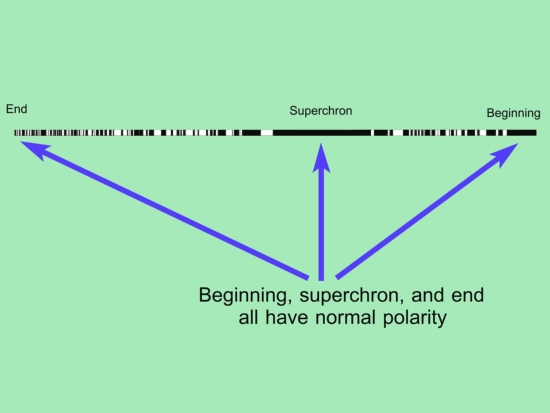
If the continents were rapidly divided and seafloor spreading occurred quickly, as described in the Shock Dynamics theory (www.newgeology.us), then the geomagnetic field would have been in a state of normal polarity at the time. Reversals would have been momentary oscillations caused by movement of the continents and the formation of mountain ranges.
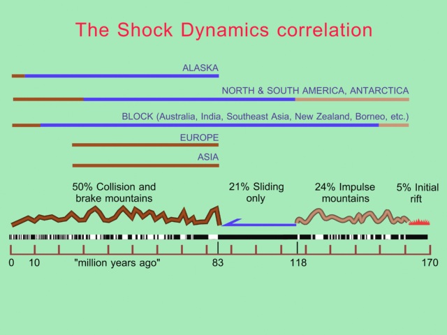
I propose that the normally-polarized geomagnetic field oscillated at the surface during the two periods of major mountain building in the Shock Dynamics theory. An analogy for illustration might be a spring-mounted gauge that oscillates when bumped but eventually returns to its starting position.
The energy of earthquakes nowadays is minuscule compared to the energy of the proposed Shock Dynamics event. Rock fracturing during the lateral crush of rapid mountain building throughout the Shock Dynamics event would have been on a colossal scale.
Fracturing of quartz and igneous rock produces piezoelectric/magnetic emissions and has been associated with earthquakes. The range of emitted frequencies is broad, and includes ultra-low (Fraser-Smith, 1990; Freund, 2002; Takeuchi, 2002; Yoshida, 2004). Widespread and massive breaking of silicate crust during compression that raised mountain ranges should produce a large piezomagnetic signal, but a study of the 2011 Tohoku earthquake and tsunami indicates that it was localized. However, a large and protracted geomagnetic oscillation was induced when the event disturbed the ionosphere (Utada, 2011). This is significant since the ionosphere surrounds the Earth.
Another study, this time of the December 2004 Sumatra earthquake, reveals the possibility that this near-surface shaking could also have affected the core-mantle boundary (CMB), leading to a "geomagnetic jerk".
"The secular variation of the core field is generally characterized by smooth variations, sometimes interrupted by abrupt changes, named geomagnetic jerks. The origin of these events, observed and investigated for over three decades, is still not fully understood." "The large Sumatra earthquake from December 2004 has revived interest in the discussion of a suggested correlation between earthquakes and geomagnetic jerks."(Mandea, 2010)
"The CMB deformation field produced by the Sumatra earthquake turns out to be comparable to that resulting from core flow processes. In particular, we have verified that the CMB deformation is of the same order of magnitude of that resulting from core torsional oscillations and it is characterized by spectral components with similar symmetry. This suggests that the global deformation field from giant earthquakes has the potential to interfere with core processes." "A perturbation of the CMB topography of seismic origin could, at least in principle, trigger a core flow instability which can lead to a geomagnetic jerk." The similarity of the deep effects of the Sumatra earthquake to conditions modelled for geomagnetic jerks suggests the possibility that the "Sumatra event could really have triggered a jerk."(Cannelli, 2007)
If this is the case, the grand-scale movements and collisions of crust during the Shock Dynamics event would have led to severe and prolonged oscillation of Earth's magnetic field.
Also, numerical earthquake simulation shows that horizontal motion of Earth's crust across the geomagnetic field generates significant electromagnetic fields by motional induction. "When a conductor moves across a magnetic field, an electomotive force or electric potential will be generated across the conductor due to the well-known Faraday's law of induction. In fact such a phenomenon also occurs during an earthquake event because of the existence of the Earth's magnetic field and the conductive property of the Earth's crust." (Gao, 2014)
While this effect was calculated from the tiny motion of crust during earthquake slip, its application to continents sliding thousands of miles is reasonable. Such sliding, as described in the Shock Dynamics event, would therefore be expected to produce enormous electromagnetic activity.
Whether the cause was primarily compression of the crust while raising thousands of miles of mountain chains in a matter of hours, or motion of landmasses across the geomagnetic field, the correlation of the Geomagnetic Polarity Time Scale with Shock Dynamics mountain building is intriguing.
Another phenomenon should be noted in passing. "It has long been known that volcanic eruptions can produce vigorous lightning." In 2006, researchers set up two stations near Mount St. Augustine in Alaska to locate the direction and intensity of impulsive radio emissions from lightning after two initial volcanic eruptions in mid-January. They recorded four explosive eruptions on 27-28 January and identified two types of emissions. The first was "a newly identified explosive phase in which the ejecta from the explosion appeared to be highly charged upon exiting the volcano, resulting in numerous apparently disorganized discharges and some simple lightning", the net charge being positive. "In the second phase, conventional lightning discharges occurred within the plume cloud produced by the explosion."(Thomas, 2007) Isolated volcanic eruptions have only a local effect. It is interesting to consider the electromagnetic effect of innumerable simultaneous eruptions globally.
Other observations
Here are excerpts from geologist David Pratt on marine magnetic anomalies from his webpage Problems with plate tectonics: reply.
"Seafloor spreading, in combination with global magnetic reversals, is supposed to produce the alternating bands of slightly higher and lower magnetic intensity on either side of ocean ridges. However, linear magnetic anomalies are known from only 70% of the seismically active midocean ridges, and the diagrams of symmetrical, parallel, linear bands of anomalies displayed in many plate-tectonics publications bear little resemblance to reality. The anomalies are symmetrical to the ridge axis in less than 50% of the ridge system where they are present, and in about 21% of it they are oblique to the trend of the ridge. Linear anomalies are sometimes present where a ridge system is completely absent, and not all the charted anomalies are formed of oceanic crustal materials. A complicating feature is that each magnetic lineation consists in detail of numerous, narrow, high-amplitude anomalies."
"Correlations
between magnetic stripes on either side of a ridge or in different parts of
the ocean have been largely qualitative and subjective, and are therefore
highly suspect.
The data are subject to significant manipulation and
smoothing, and virtually no effort has been made to test correlations
quantitatively by transforming them to the pole (i.e. recalculating each
magnetic profile to a common latitude). The magnetic anomalies of the
Reykjanes Ridge are supposed to be a classic example of ridge-parallel
symmetry, but Agocs et al. (1992) concluded from a detailed, quantitative
study that the correlations were very poor. The distance between bands of magnetic anomalies is
not proportional in most cases to the length of the geomagnetic epochs. The
lengths of the Brunhes, Matuyama, and Gauss epochs have the ratio 1.0 : 2.4 :
1.6. However, on the Reykjanes Ridge, the distances between the
anomalies closest to its axis have the ratio 1.0 : 0.5 : 0.4. An equally
great breach of proportionality is observed on the East Pacific Rise, which
can be explained from the angle of plate tectonics only by invoking
considerable changes in the spreading rate.
Asymmetric seafloor spreading frequently has to be invoked as well."
"The initial, highly simplistic seafloor-spreading model for the origin of ocean magnetic anomalies has been disproven by ocean drilling (Hall and Robinson, 1979; Pratsch, 1986). First, the hypothesis that the anomalies are produced in the upper 500 metres of oceanic crust has had to be abandoned. The existence of different polarity zones at different depths suggest that the source of magnetic anomalies lies in deeper levels of ocean crust not yet drilled or dated. Second," there are "vertically alternating layers of opposing magnetic polarization directions. Given that the magnetic-stripe timescale is probably fictional, any correspondence between plate-motion estimates derived from it and space-geodetic data is likely to be either coincidental or the result of biased interpretation."
***********
References
Agocs, W.B., Meyerhoff, A.A., and Kis, K. 1992. Reykjanes Ridge: quantitative determinations from magnetic anomalies. In Chatterjee, S. and Hotton, N., III, eds., New Concepts in Global Tectonics, Lubbock, TX: Texas Tech University Press, pp. 221-238.
Cande, S.C. and D.V. Kent. 1995. Revised calibration of the geomagnetic polarity time scale for the Late Cretaceous and Cenozoic. Journal of Geophysical Research, Vol. 100, No. B4, pp. 6093-6095.
Cande, Steven C., Dennis V. Kent. September 10, 1992. A New Geomagnetic Polarity Time Scale for the Late Cretaceous and Cenozoic. Journal of Geophysical Research, Vol. 97, No. B10, pp. 13,917-13,951.
Cannelli, V., D. Melini, P. De Michelis, A. Piersanti, F. Florindo. 2007. Core-mantle boundary deformations and J2 variations resulting from the 2004 Sumatra earthquake. Geophysical Journal International, Vol. 170, pp. 718-724.
Fraser-Smith, A.C., A. Bernardi, P.R. McGill, M.E. Ladd, R.A. Helliwell, O.G. Villard, Jr. August 1990. Low-frequency magnetic field measurements near the epicenter of the Ms 7.1 Loma Prieta earthquake. Geophysical Research Letters, Vol. 17, No. 9, pp. 1465-1468.
Freund, Friedemann. 2002. Charge generation and propagation in igneous rocks. Journal of Geodynamics, Vol. 33, pp. 543-570.
Gao, Yongxin, Xiaofei Chen, Hengshan Hu, Jian Wen, Ji Tang, Guoqing Fang. 2014. Induced electromagnetic field by seismic waves in Earth's magnetic field. Journal of Geophysical Research: Solid Earth, Vol. 119, pp. 1-35 DOI:10.1002/2014JB010962
Gee, J., D.A. Schneider, D.V. Kent. 1996. Marine magnetic anomalies as recorders of geomagnetic intensity variations. Earth and Planetary Science Letters, Vol. 144, pp. 327-335.
Gubbins, David. 1999. The distinction between geomagnetic excursions and reversals. Geophysical Journal International, Vol. 137, pp. F1-F3.
Hall, J.M., P.T. Robinson. 1979. Deep crustal drilling in the North Atlantic Ocean. Science, Vol. 204, pp. 573-586.
Lanci, Luca, William Lowrie. 1997. Magnetostratigraphic evidence that 'tiny wiggles' in the oceanic magnetic anomaly record represent geomagnetic paleointensity variations. earth and Planetary Science Letters, Vol. 148, pp. 581-592.
Liebke, U., E. Appel, U. Neumann, L. Ding. 2012. Dual polarity directions in basaltic-andesitic dykesreversal record or self-reversed magnetization? Geophysical Journal International, Vol. 190, pp. 887-899.Lowrie, William. 1979. Geomagnetic Reversals and Ocean Crust Magnetization. in Deep Drilling Results in the Atlantic Ocean: Ocean Crust, eds. Manik Talwani, Christopher G. Harrison, Dennis E. Hayes, American Geophysical Union, pp. 135-150.
Mandea, Mioara, Richard Holme, Alexandra Pais, Katia Pinheiro, Andrew Jackson, Giuliana Verbanac. 2010. Geomagnetic Jerks: Rapid Core Field Variations and Core Dynamics. Space Science Reviews, Vol. 155, pp. 147-175.
Pratsch, J.C. July 14, 1986. Petroleum geologist's view of oceanic crust age. Oil and Gas Journal, Vol. 84, pp. 112-116.
Roberts, Andrew P. 2008. Geomagnetic excursions: Knowns and unknowns. Geophysical Research Letters, Vol. 35, L17307, 7 pages.
Smith, Norm, Jane Smith. 1993. An alternative explanation of oceanic magnetic anomaly patterns. Origins, Vol. 20, No. 1, pp. 6-21.
Takeuchi, Akihiro, Hiroyuki Nagahama. 2002. Interpretation of charging on fracture or frictional slip surface of rocks. Physics of the Earth and Planetary Interiors, Vol. 130, pp. 285-291.
Thomas, R.J., P.R. Krehbiel, W. Rison, H.E. Edens, G.D. Aulich, W.P. Winn, S.R. McNutt, G. Tytgat, E. Clark. 23 February 2007. Electrical Activity During the 2006 Mount St. Augustine Volcanic Eruptions. Science, Vol. 315, p. 1097.
Tivey, Maurice A., H. Paul Johnson, Corinne Fleutelot, Stefan Hussenoeder, Roisin Lawrence, Cheryl Waters, Beecher Wooding. October 1, 1998. Direct measurement of magnetic reversal polarity boundaries in a cross-section of oceanic crust. Geophysical Research Letters, Vol. 25, No. 19, pp. 3631-3634.
Utada, Hisashi, Hisayoshi Shimizu, Tsutomu Ogawa, Takuto Maeda, Takashi Furumura, Tetsuya Yamamoto, Nobuyuki Yamazaki, Yuki Yoshitake, Shingo Nagamachi. 2011. Geomagnetic field changes in response to the 2011 off the Pacific Coast of Tohoku Earthquake and Tsunami. Earth and Planetary Science Letters, Vol. 311, pp. 11-27 DOI:10.1016/j.epsl.2011.09.036Valet, Jean-Pierre, Guillaume Plenier, E. Herrero-Bervera. 2008. Geomagnetic excursions reflect an aborted polarity state. Earth and Planetary Science Letters, Vol. 274, pp. 472-478.
Yang, Tianshui, Masayuki Hyodo, Zhenyu Yang, Huidi Li, Makoto Maeda. 2010. Multiple rapid polarity swings during the Matuyama-Brunhes transition from two high-resolution loess-paleosol records. Journal of Geophysical Research, Vol. 115, B05101, 17 pages.
Yoshida, Shingo, Tsutomu Ogawa. 2004. Electromagnetic emissions from dry and wet granite associated with acoustic emissions. Journal of Geophysical Research, Vol. 109, B09204, 11 pages.
John Michael Fischer, 2006-2020
www.newgeology.us
![]()